My most recent blog topics have had to do with Wave Soldering Machine Components, but statistics is also something that interests me. Have you ever had to compare two or more sets of data to try and understand if they were unrelated or statistically significant? I recently had to solve this problem for myself by comparing variables from two different SMT assembly machines.
This is the first time that I had to use statistics since I took the course in college, so I had to brush up on a few things. The particular test that I needed to perform was unclear to me at the start of the analysis. Let me say that the machines were measuring the exact same variable, the only difference was the machine. I wanted to understand which machine was more accurate. Or, better yet, if there was a statistically significant difference between the two sets of results. Let’s start off with the definition of “statistically significant.” According to Google, the definition of statistically significant is. "the likelihood that a result or relationship is caused by something other than mere random chance. Statistical hypothesis testing is traditionally employed to determine if a result is statistically significant or not.”
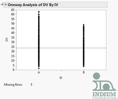
After some research, I found that I could use either the t-test or the analysis of variance (ANOVA) test. The t-test looks at differences between two groups using a single variable while the independent variable must only have two groups. The ANOVA analysis tests the significance of differences between two or more groups of data. The independent variable has to have two or more categories. The ANOVA only determines that there is a difference between groups, but doesn’t tell which is different. Strangely enough, if you perform the ANOVA analysis for two independent variables you create the same result as using the t-test. Here is a snap shot of what my data looks like:
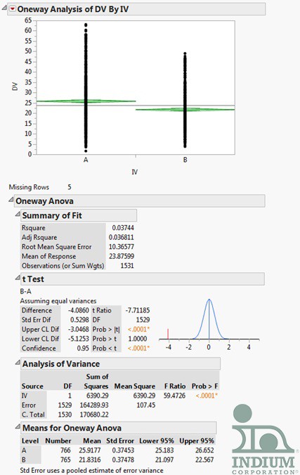
After using the JMP software and turning on the ‘Means/ANOVA/Pooled t', my data now looks like this:
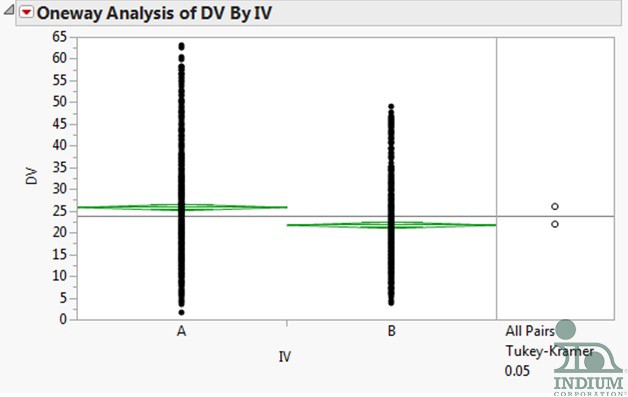
According the JMP support page, “The Prob > F value measures the probability of obtaining an F Ratio as large as what is observed, given that all parameters except the intercept are zero. Small values of Prob > F indicate that the observed F Ratio is unlikely. Such values are considered evidence that there is at least one significant effect in the model.” This data fits the description, so I used a secondary test, the Tukey-Kramer test, to verify my results. When you select this test the image of the data changes slightly to this:
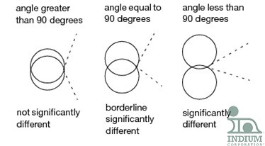
When I first employed this test I did not fully understand what the circles represented. Here is the most comprehensive graphic that I found.
Because the circles do not overlap at all the results are significantly different.
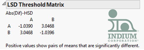
There is also a least significant difference or LSD Threshold Matrix that pops up when you select the Tukey-Kramer analysis. It is displayed below:
The way to read the matrix is, when you compare A to B, there is a positive number indicating that the pair of means is significantly different.
From time to time I will be sprinkling in posts that are different from my standard program of fluxers, preheaters, etc. to discuss other topics or experiments that I have conducted here at the Indium Corporation. Please feel free to reach out and contact me with any questions, concerns, or fun facts. (I love fun facts!!!) I am always open to new ideas and concepts.


